Introduction
This project is to test the performance of Ipopt and Snopt in large scaling strong nonlinear optimization
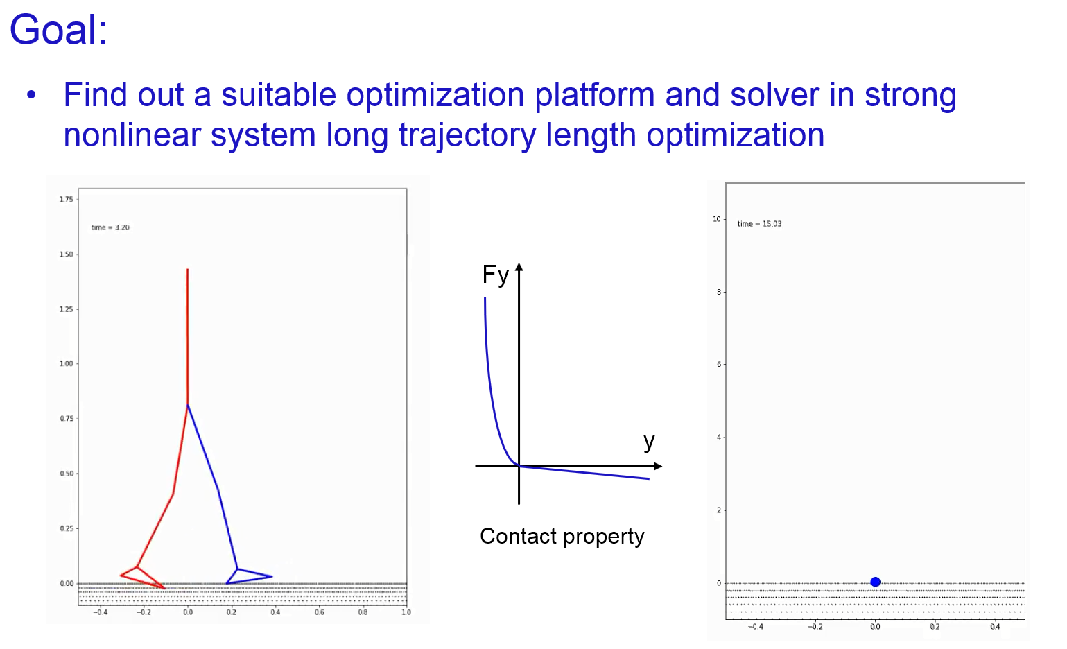
The original of this project is to find out a good solver for large scaling strong nonlinear optimization in human walking. To make the model simpler and easy understandable, Ball Bouncing system was created, which has the simplest mathematical model and strong nonlinear landing property.
Method
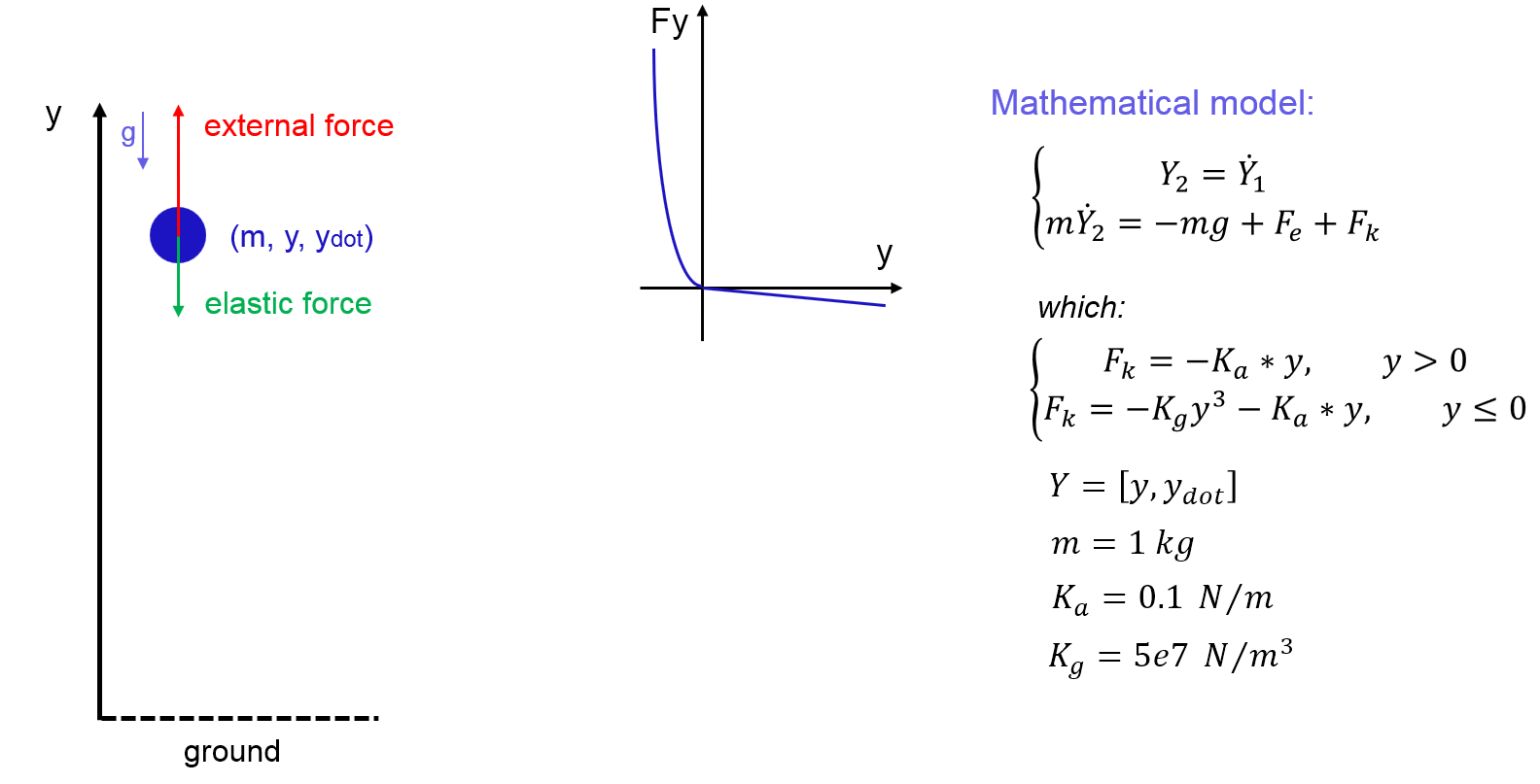
Dall Bouncing Dynamics
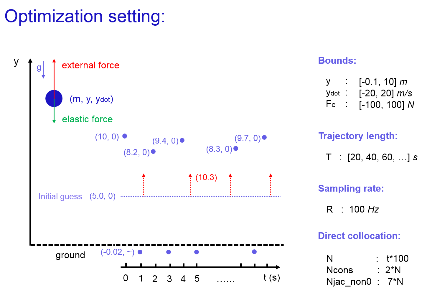
The motion dynamics of one dimensional ball is a simple second order system, but with strong nonlinear contact model. External force was applied on the ball to control moving trajectory. Contact Model is consist with two parts. When displacement of the ball is negative (contacted with ground), contact force is proportional to the third order of the displacement. When displacement of the ball is positive (in the air), a small elastic force is also applied which is proportional to the displacement. This small elastic property is helpful for gradient based optimization to converge.
Optimization Define and Settings
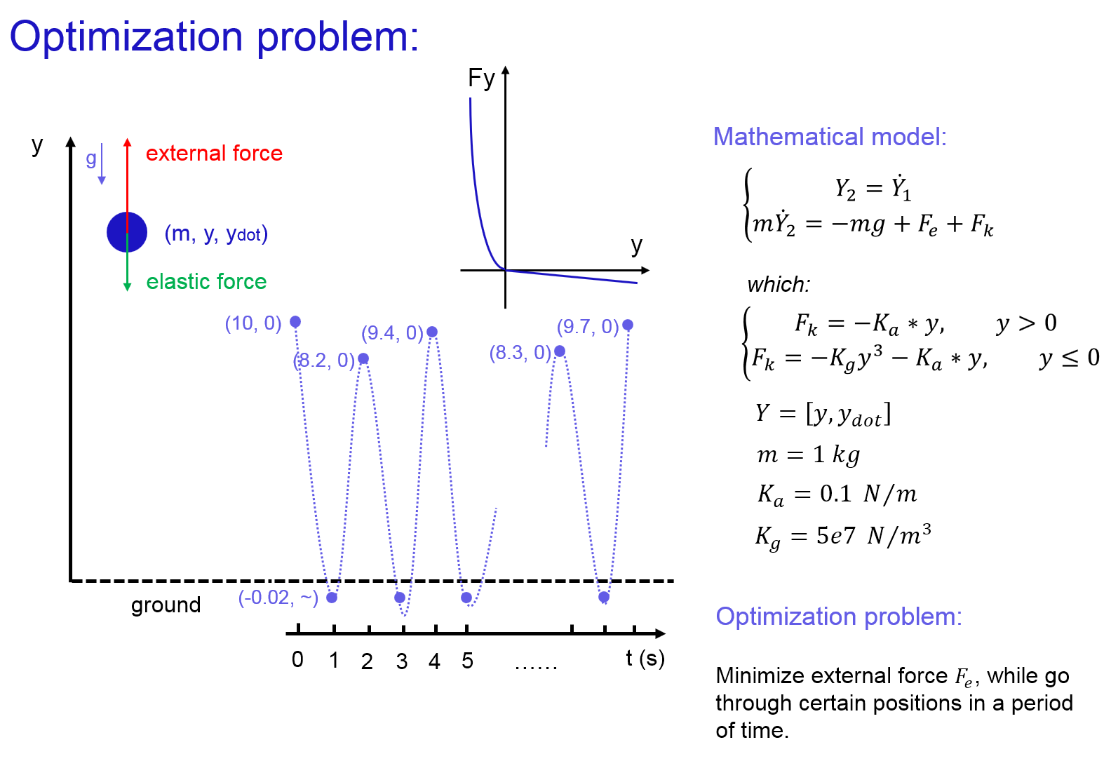
The optimization problem of Ball Bouncing is defined as minimizing the sum-square external force while enable the ball go through predefined targets. There are two kinds of targets: Peak targets and Bottom targets. Peak targets are points that the ball will reach these points with velocity zero. Peak targets are randomly defined between 8 and 10 meters. The ball should reach these peak targets at odd time seconds. Bottom targets are points that the ball will reach these points with any velocity. Bottom targets are constantly defined as -0.02 m. The ball should reach these bottom targets at even time seconds.
Optimization Solvers
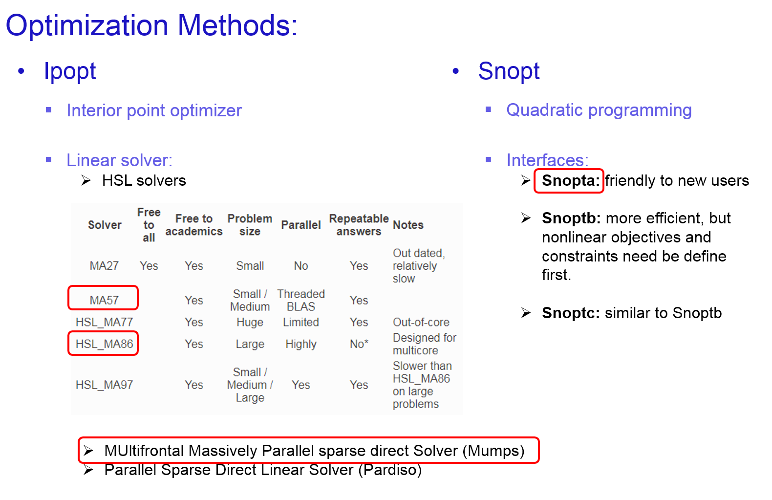
Ipopt and Snopt are used in this project to solve this large scaling problems, which could have millions of non-zero elements in Jacobian.
In Ipopt, there are several linear solvers that can be used. For instance, MA series in HSL packages, MUMPS, Pardiso. In Snopt, different interfaces can be selected to solve the problem. SnoptA is suitable for beginners, since it does not require user to define nonlinear constraints first. SnoptB is more complex than SnoptA, since it require user to define nonlinear constraints before all linear constraints. The advantage of SnoptB is that it is faster than SnoptA, since it will trying to satisfy nonlinear constraints first.
In this project, MA57, MA86, MUMPS, and SNoptA were chosen as solvers.
Result
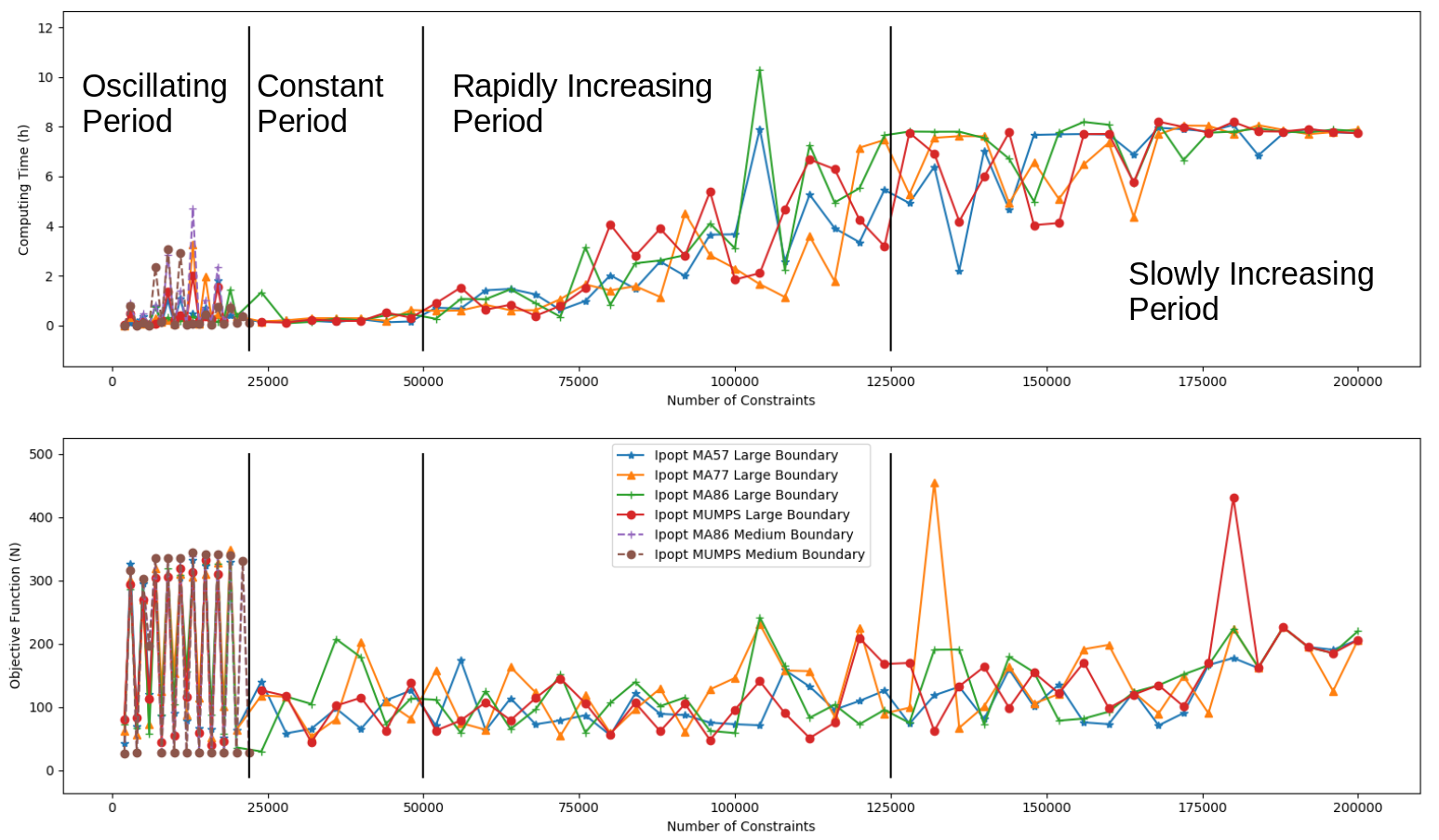
Time cost of different solvers in solving different bouncing trajectory length is shown below. Below 100 seconds optimization trajectory, time consuming is gradually increasing in Ipopt linear solver. Above 100 seconds optimization trajectory, time consuming increased rapidly.